
Say you want to give an orange an MRI scan. You pop it in the scanner, apply your radiofrequency pulse, and receive the signal. This signal will differ depending on which part of the orange it comes from, for example whether it is the flesh or the peel. But how would you be able to tell where the different types of signal come from? How would you tell that the peel signal is coming from the surface and the flesh signal from inside? In my previous post, I outlined what happens during an MRI scan. Here, I will (briefly) explain how we can tell which signal comes from which place in the object that we are scanning. This has to do with gradients.
Gradients. Gradients are additional magnetic fields that we apply to specify the location that we want to image. These fields vary slightly from the main magnetic field. The resulting overall field (the main field plus the gradients) now contains variation. Specifically, it changes linearly with distance. Protons will experience different fields depending on where they are in the object, and as a result, they have different frequencies. In other words, we get a different signal from the protons depending on where they are in the object that we image.
We have two types of gradients that we employ: frequency-encoding gradients and phase-encoding gradients.
Frequency encoding is quite simple. We take our original field (B0), add a gradient field (Gf), and we get a new field (Bx) for any given point (x) in space. Like this: Bx = B0 + xGf
The spin frequency of the protons depends on their position along this new field. The frequency at point x is the sum of the frequency induced by the main field, and that induced by the new gradient. We can now differentiate between signal from different parts of the brain to some extent (see image below).
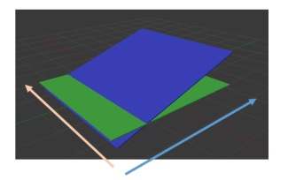 When we add a frequency encoding gradient (blue) to our main field (green), we can differentiate between signal along this gradient axis (blue arrow). We cannot tell the difference between signal along the other axis (red arrow).
To complete the picture, we need to add phase encoding gradients. We do this by applying another gradient designed to make signal fall out of sync along the phase encoding direction (red arrow axis in the image above). Although the frequency of the signal remains the same, the new gradient will cause it to have a different phase depending on where it comes from (along the red arrow axis). Think of it as a long line of cars waiting at a red light, all in sync. The light turns green, and the first car starts, then the second, then the third, and so on. Now, the cars are out of sync: some are standing still, others are slowly moving, and the first cars are moving at full speed. Also, at the same time, the cars at the back of the queue have become tired of waiting and start reversing (first the one all the way at the back, then the next one, and so on). The full speed profile of the row of cars suddenly has a great deal of variation, with some going forward at different speeds and some going backward at different speeds. In terms of MRI, the shift in phase causes the sum of the frequencies (the sum of the car speeds) along the red arrow axis to vary, and we can use this variation to figure out the individual signals (or individual cars) along the axis.
Through these frequency and phase encoding steps, we can figure out the strength of the signal and location of signal along both axes.
Frequency vs Phase Encoding. An important difference between frequency encoding and phase encoding is speed. Frequency encoding can be done with a single radiofrequency pulse (see my previous blog post on what happens during an MRI). We apply a gradient and a pulse, and all the frequencies can be read all at once. It is fast. For phase encoding, we need to apply a radiofrequency pulse for each phase change. We apply our pulse and then the gradient, let the phase change happen, measure the change, and then we have to apply another gradient and phase change. For a 256 pixel image, we will have to do this 256 times, each taking as long as one TR (repetition time). It is slow. A consequence of this is that the phase encoding is more vulnerable to movement than the frequency encoding.
In my next blog post, I will describe how we store the MRI signal during the scan and how the signal can be transformed into an image.
