Measuring brain blood flow

Brain blood flow can be measured in many ways, but in this post I will focus on transcranial Doppler ultrasound (TCD). This method is used to measure the speed and direction of blood flow through a single blood vessel in your head.

TCD is a great measure for brain blood flow: the method can measure blood flow beat-by-beat (we tend to say that it has excellent temporal resolution – it collects a lot of data points per unit time). It is also non-invasive, meaning it causes no harm to the body (although a lower power should be used for some probe placements). It is very good for measure changes in blood flow, for example due to certain stimuli, and can be used to measure how well blood flow responds to such stimuli.

So what is this signal? What happens when we use ultrasound is that an ultrasonic beam is sent from the probe and into the blood vessel, where it is reflected back from the moving red blood cells. The returned signal is slightly different from the first signal. If the blood cells are moving towards the probe, the returned signal has a higher frequency. If it is moving away from the probe, the returned signal has a lower frequency. How much of a faster or lower signal depends on how fast the blood cells move. We call this change in wavelength the Doppler shift or the Doppler effect, and it has the symbol f. It is this Doppler shift that is being used to calculate blood flow velocity.

Most of us have seen the Doppler shift in action. A common example is if an ambulance or fire engine passes us in the street with its sirens on. When it comes towards us, the source of the sound (the vehicle) is moving in the same direction as the sound of the siren, and the sound waves are therefore compacted (have a shorter wavelength), resulting in a higher frequency sound (a higher pitch). When it has passed us and moves away, the vehicle moves in the opposite direction to the sound of the siren (relative to us) and so the sound waves are stretched (have a longer wavelength), we get a lower frequency sound (a lower pitch).

(Not clear? Here is a Vimeo video illustrating the Doppler effect and the example above)

Ok, which blood vessel is best. There are plenty of blood vessels in the brain, but the middle cerebral artery (MCA) is great as it is a major artery and easy to locate. The MCA emerges from the carotid artery, which is the main artery going to the head. We have one carotid artery on each side of the neck (which you can feel when you take your pulse). At the top of the neck, the carotid artery divides in an internal and an external branch. The internal branch then divides into the MCA and the anterior cerebral artery (ACA). The MCA receives around 70% of the internal carotid artery blood flow, and we therefore often assume that blood flow through the MCA is representative of the total blood flow to one half of the brain.

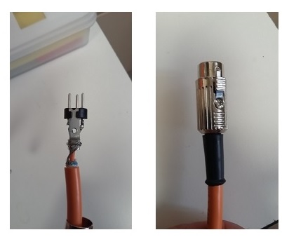
How to measure the flow. When we image blood flow through this vessel using TCD, we put the ultrasound probe to a person’s temple, and choose an ultrasound beam depth at around 45-60 mm. The best depth depends on the anatomy of the person – there is a bit of variation in the population, so you may have to try different depths to get a good signal. The temple is a good place to measure blood flow, as it is where the internal cerebral artery splits into the ACA (blood flowing away from the probe) and the MCA (blood flowing towards the probe). This gives a very distinct waveform (see below) and means we can be reasonably sure we have placed the probe and the ultrasound beam correctly.

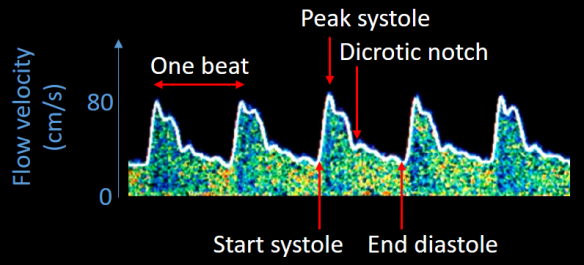
Typical TCD trace from the middle cerebral artery. 

It should be mentioned that when measuring blood flow through other vessels, we may choose a different placement of the probe. This can include putting the probe over the (closed) eye (transorbital), at the base of the neck (suboccipital) or on the neck below the ear (submandibular). We call these placements ‘windows’ (i.e. the transtemporal window is the placement of the probe on the temple). From the transtemporal window, we can see flow through the MCA, ACA, the terminal internal cerebral artery (ICA) and the posterior cerebral artery (PCA).

What is the physiology behind the signal? The waveform shows changes in blood flow due to systolic and diastolic phases of the heart. Referring to the image above, each one of the ‘waves’ is a heartbeat. The start of the systole, peak systole, dicrotic notch and the end of the diastole are marked on the figure. Systole is when the heart contracts and pumps the blood out, and diastole is when the heart relaxes and refills with blood. The dicrotic notch is a short-term change in aortic pressure that stems from the closure of the aortic valve. This valve is between the left ventricle of the heart and the aorta, and blood passes this valve as it enters the body circulation. 

So it starts with the beginning of the systole (when the heart starts to contract). The increased pressure in the contracting heart pushes blood out of the left ventricle and into the circulation through the aorta. Some of this blood goes to the brain and is what we measure with TCD. Blood flow increases through the blood vessels as it is being pumped out of the heart. At peak systole, the blood flow for that particular heartbeat is at its maximum. Then, as the heart begins to relax, the pressure in the ventricle drops and it begins to refill with blood (coming from the lungs). The aortic valve closes and stops blood from flowing the wrong way back into the heart. This closure of the valve can be seen as a small change in blood flow (the dicrotic notch). We reach the lowest flow just as the heart is filled up and ready to contract again. TCD gives us a measure of the blood flow at all these stages of the cardiac cycle.

Ultrasound of the heart. All four heart chambers are visible, as are the valves (flapping open and closed) between the atrial and ventrical chambers.

The temporal resolution of TCD is excellent. As can be seen in the gif above, ultrasound lets us see things in more or less real time (in this case a beating heart), and this makes it a useful technique for measuring rapid changes in brain blood flow.

I will be posting a short tutorial on how to analyse TCD data soon, and if anyone has any questions on the method before then, I would be happy to address them in the comments.

How small is too small? MRI of tiny structures

MRI is great for imaging tissues and organs, as it does not involve any invasive procedures (such as drugs, radiation or even needles/scalpels). It allows us to quickly and safely get a good idea of what goes on under the skin. However, just as with a photo, it can become pixelated and useless, especially if you are looking at small structures. Imagine taking a holiday snapshot of a distant landmark, say, the Eiffel tower, but when you zoom in, it becomes hard to see what is tower and what is sky. Up close, the image is hard to interpret, and determining the exact size of the structure in the image may become impossible. In a pixelated image of the Eiffel tower, one pixel may contain both tower and sky, and you can’t tell where the exact line between the two goes. This is also the case with MRI.

The MRI image is divided into voxels (same as pixels, just three-dimensional – think of it as a set of tiny cubes making up the image). The quality of your image depends on the number of voxels and the signal from these. Too few voxels, not enough information. It would be like having just a few pixels covering the spire of the Eiffel tower – it won’t look good. One voxel covering a big chunk of the brain of a human participant won’t be very useful as there simply is not enough resolution to determine what’s what.

You can also have enough voxels but too little signal. Too little signal means not enough information. It would be like taking the photo without any light. In photography, light creates the image. If you have plenty of light, you can typically get more detail from each part of your image, and so your resolution can be better. Not enough signal means you need to keep your shutter open for longer, to let more light in. You can do that, but you probably need a tripod, and any movement (birds, people, wind, clouds, a bus rumbling past) will affect your picture and make it blurry. Same with MRI. You can increase signal by increasing scan time, but that’s not always possible and means you have to keep people still and in the scanner for longer.

Typically, the stronger your field strength, the more signal (light) you can get from your voxels. More signal means you can reduce voxel size as you will be getting more detail from each part of your scan. This typically results in better resolution. Or, you can get the same resolution, just faster (i.e. keep the shutter open for a shorter period). This can be useful if what you’re wanting to scan moves. For some tissues, it is invaluable to be able to get quick images. Imagine getting an image of a beating heart, for example. You need a quick scan sequence, and you typically need to do it several times over to get a nice, detailed image. That is the equivalent of taking lots of quick shots of the Eiffel tower (swaying in the wind, perhaps), and piecing them together to get all the fine details. This process of getting many snapshots of the same thing and taking the average to get a good image is very common in MRI, and it helps with a third issue: noise.

Everything you see in an MRI image is either signal, or it is noise. We call the relationship between signal and noise a signal-to-noise ratio (SNR), and we want it to be as high as possible (more signal, less noise). Noise in MRI images is usually caused by particles with an electrical charge moving around slightly in the human body, or by electrical resistance in the MRI machine itself. Together, these cause variations in signal intensity. Again, in our photo of the Eiffel tower, this is much the same: small visual distortions that gives it a grainy quality.

When we have smaller voxels, we typically get less signal and more noise per voxel (a low SNR). The way around it is to increase the number of averages that we run – i.e. take more snapshots, get a better image. Unfortunately, this takes time. Usually, then, we end up with a compromise of how good a resolution we want and how long we want the scanning to take, and this is greatly dependent on the kind of signal we can get.

The good news is that signal is, as mentioned earlier, grossly dependent on the field strength of our magnet. And we have some strong magnets available to us. For a human scan with a field strength of 3 Tesla (T), a resolution of 1mm x 1mm is easily obtained in about 5 minutes. That is fine for a structural scan of, say, a human brain. But what if you want to scan something smaller? Humans move, no matter how hard they try not to, even if it is only to draw breath. Higher resolutions means you’ll pick up on these small movements. A tiny motion can shift a small voxel completely out of place, while a bigger voxel would be less affected. In short, smaller makes things more difficult.

So, how small is too small?

For higher-field machines in humans, such as 7T, you can go small. 0.5mm x 0.5mm for 7T is easily doable, and some post mortem scans has gone down to 0.14mm x 0.14mm [1]. For our 9.4T scanner, we have scanned with resolutions of 0.03mm x 0.03mm (post mortem), and resolutions at 0.06mm x 0.06mm should be possible for scans that are not post mortem. That means with 9.4T, we can in theory image structures as small as 0.25mm across with some clarity (remember, you need to have at least a few voxels of the thing you want to image to properly see the edges and detail of it). Our scanner is too small for a whole human, but there exists 9.4T MRI machines for humans. And an 11.75T magnet is underway (see the BBC news story here), which will be able to get resolutions down to 0.1mm (or possibly more) in humans. So at present, anything less than 0.25mm is probably too small for MRI.

Smaller than that, and we have to use other methods. Microbiologists and their microscopes are likely to laugh in the face of 0.25mm. Below is a picture with a 9.4T image and histology image of testicular tissue [2], showing how much detail both techniques afford. Histology is obviously better. Sadly, however, it still requires scalpels, and MRI does not.

References:
[1] Stucht D, Danishad KA, Schulze P, Godenschweger F, Zaitsev M, Speck O. Highest Resolution In Vivo Human Brain MRI Using Prospective Motion Correction. PLoS ONE. 2015;10(7):e0133921. Link: https://www.ncbi.nlm.nih.gov/pmc/articles/PMC4520483/
[2] Herigstad M, Granados-Aparici S, Pacey A, Paley M, Reynolds S. Imaging seminiferous tubules – a 9.4T MRI mouse model. bioRxiv 155762; Link: https://doi.org/10.1101/155762

The wiring of DIN plugs

I get to do all sorts of practical stuff at work, some of which has nothing to do with physiology or imaging. One such thing is producing custom-made cables and plugs. Since I’ve had the pleasure of doing a fair few of these recently, I thought I’d put up a short how-to blog post on wiring up a DIN connector.

DIN stands for Deutsches Institut fur Normung, which translates to the German Institute for Standardisation. A DIN connector is, in short, a standardized connector, which come in a similar size. You may have seen them as they are often used for analog audio. The male DIN plug is typically 13.2 mm in diameter, and it often has a notch at the bottom to make sure the plug goes in the right way. Male plugs have a set of round pins, 1.45mm in diameter, that are equally spaced within the plug. The different types of DIN plugs have different numbers and configurations of pins. Below is an overview of some typical pin configurations.

There are, of course, variations over these themes, as well as specialized plugs with more than 10 pins. Pins on male connectors are numbered. The numbering* goes from right to left, viewed from the outside of the connector with the pins upward and facing the viewer. The female counterparts are the inverse of the male plugs, and their numbering is from left to right. Usually, only corresponding male-female pairs work together, but you may be able to fit a 3-pin plug with a 5-pin 180 degree plug.

*EDIT: to clarify, the numbering of the pins are not in order, as pointed out in the comments (thank you!). For the plugs, a 5-pin plug would be numbered (from right to left for the male, and from left to right for the female): 1–4–2–5–3.

So how to attach a DIN plug to a cable? 

1. Take the cable and snip off a few centimetres of plastic and remove padding. Snip off the insulation (about 1 cm) of the individual internal cables (cores). Slide the DIN metal sheet over the wire.
2. Make sure that each core fits neatly into holes of DIN plug. This might mean cutting some of the wires. Move the unisolated wires (the ground) to one side.
   
3.  Solder the core wires together and test that they still fit the holes in the plug.
4. (Now comes the fiddly part). Add solder tin (a small amount is best) to the DIN plug holes, heat with the solder and push the tinned cores into holes. Remove solder iron and let the tin solidify (a few seconds only). Test that the solder holds by pulling firmly on the plug and cores. Attach the metal clamp around the cores (see second of figures below).
   
5. Wrap the ground wires around the base of the metal clamp. Make sure the ground does NOT touch the cores. Test that there is no connection between wires and between wires and ground using a multimeter. Slide the metal sheet over the structure and plastic, and screw on the release catch where this overlays hole on metal clamp.
   

Done.

Reblog: Electrical shavers and splashed saline

One morning, your friend and you go to a café and get two identical coffees. Without telling you, a barista gives you a regular coffee and your friend gets a decaf. This means you are blinded to whether your drink contains caffeine or not.

I recently had the pleasure of being asked to give feedback on a blog post on blinding in clinical trials, and how this can be done if the trial involves surgery. It was a really interesting read, highlighting how creative you have to get to conceal real versus fake surgical interventions.

For anyone interested, the full post has just been released here.

For anyone very interested, the review paper that the blog post was based upon is here.